In this project we were supposed to select an interesting project from a list of potential projects that involve a certain amount of advanced statistic. The projects were mostly ArcGIS tutorial projects with some additional analysis included. For my project I elected to explore kriging interpolation using the geostatistical analyst extension in ArcGIS. Primary data was collected from the California Air Resource Board and contains measured ozone concentrations for specific hour of 3-4pm on September 6th 2006. From these discrete data I interpolated a surface of ozone concentration using both a default (Fig. 1) and trend removed kriging (Fig. 2). I identified trends and directionality in the data to reduce the error in the prediction. A second order polynomial was removed and a northwest-southeast trend in similarity was accounted for. Error is compared both quantitatively and qualitatively via mapping (Fig. 3) and statistically (Fig. 4). The geostatistical analyst also allows for probability interpolation which was used to see the probability that ozone values crossed a threshold of 0.09 ppm (Fig. 5). Finally I compared the used of the use of the geostatistical analyst extension to other interpolation techniques built into ArcGIS (Fig. 6).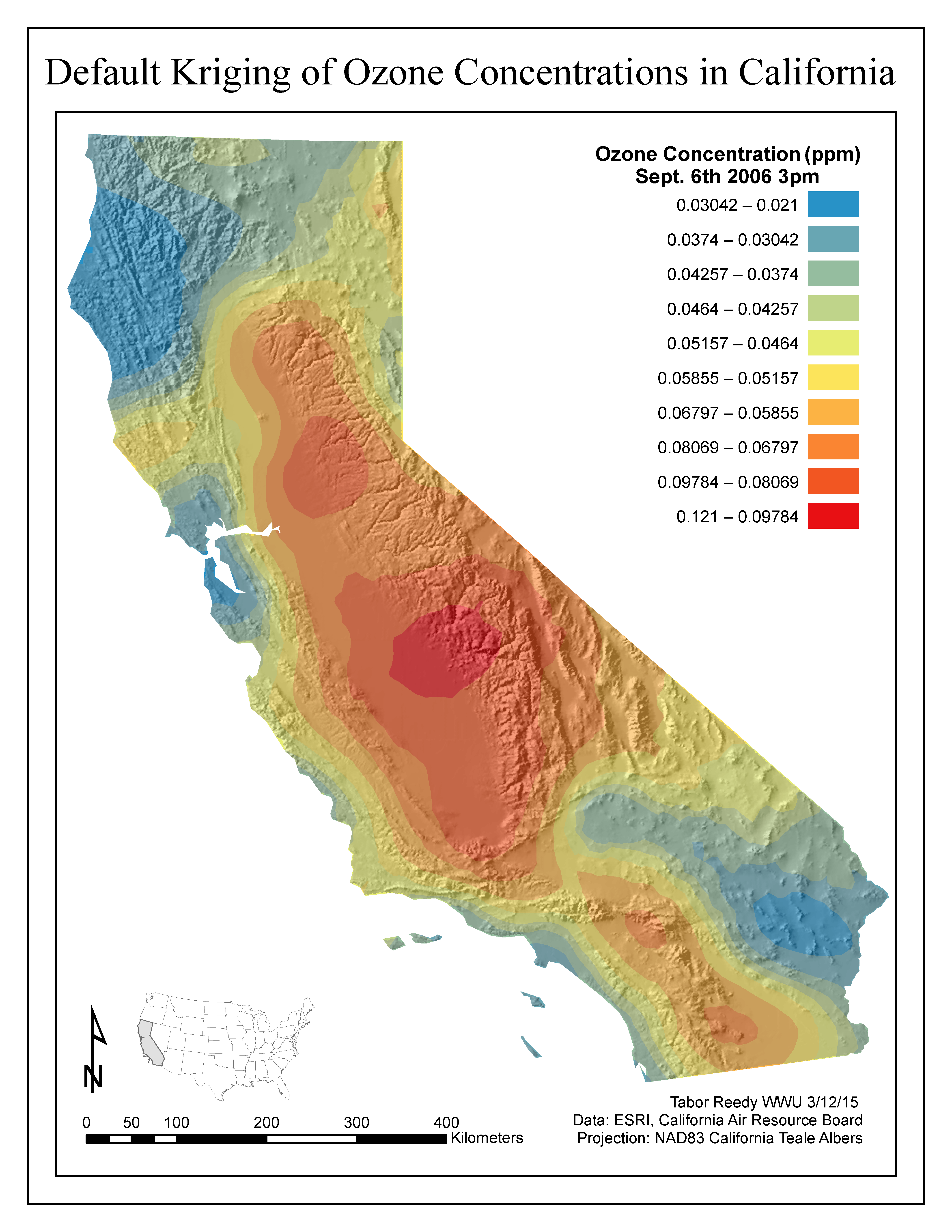 Figure 1. This map of ozone concentrations in California was created using default parameters in the geostatistical analyst extension in ArcGIS. Air testing locations were used with a kriging interpolation to create a continuous surface of predicted values. Kriging is a form of Gaussian regression governed by prior covariance. No trend is removed to account for directionality of the data distribution.
 Figure 2. This map of ozone concentrations was created using a kriging interpolation with a second order polynomial trend removed and the neighborhood to weigh values adjusted for directionality of the data. This means the distribution generally accounts for high concentrations in the Central Valley, and low concentrations due to elevation in the mountains and wind on the coast.
 Figure 3. Objective standard error predictions based on distributions of data compared to a normal distribution of data. Interpolation techniques are best suited to normal distributions of data. By removing trends and adjusting for directionality, the trend removed surface is clearly more accurate.
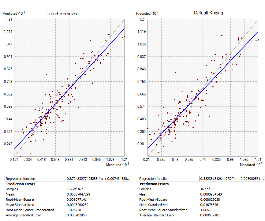 Figure 4. Distribution of data and the standard error associated with each interpolation. The trend removed kriging shows more accuracy, and the average line (blue) is closer to the linear normal distribution of data.
 Figure 5. Probability that any area exceeded 0.09ppm over the 3-4pm time period on September 6th 2006. The interpolated surface is the trend removed kriging surface. Probability is calculated using an indicator kriging with a probability output. Kriging interpolation generated using the geostatistical analyst extension in ArcGIS.
 Figure 5. Probability that any area exceeded 0.09ppm over the 3-4pm time period on September 6th 2006. The interpolated surface is the trend removed kriging surface. Probability is calculated using an indicator kriging with a probability output. Kriging interpolation generated using the geostatistical analyst extension in ArcGIS.
Full Report: Reedy_Lab6_Report
